Simple features

I spent this week playing around with generation and visualisation of simple malware features obtained through signatures JSON field. This field contains some high level binary descriptions provided by Cuckoo Sandbox analysis. This field among others contains a tag and its description. All these tags come from a finite set, hence, they can be used as binary (true/false) features for the analysis. They also belong to variety of categories, therefore, they can be grouped and clustering can be performed on particular group rather than the whole set. These groups have been hand crafted and are available in modules/cuckooml/cuckooml.py file at the top of ML class. These need to be double-checked to ensure robustness.

Visualisation

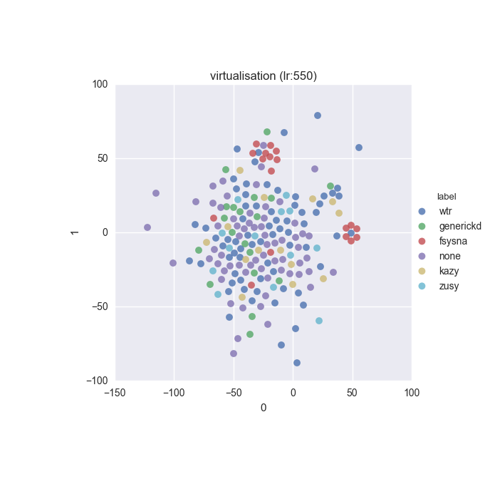
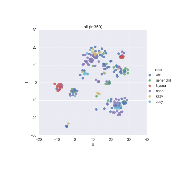
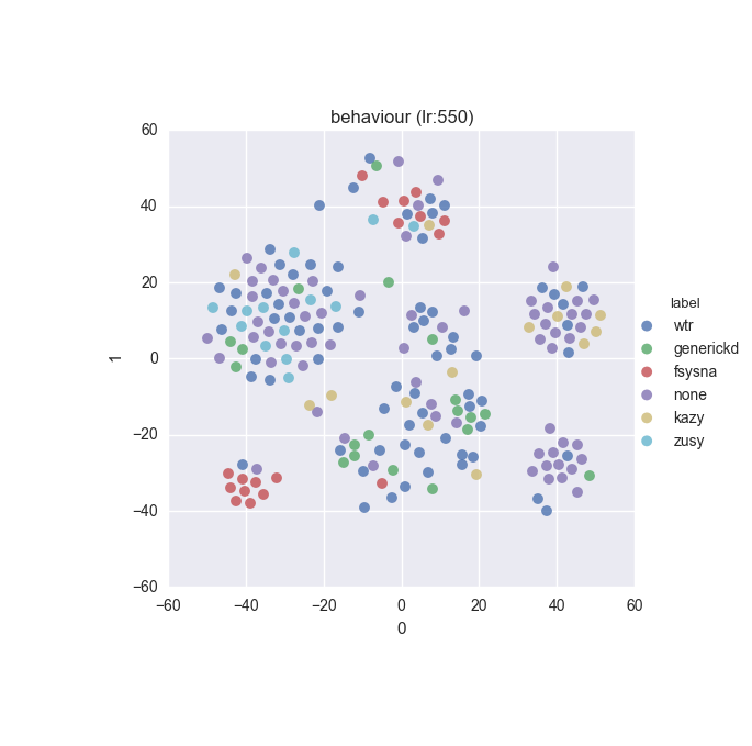
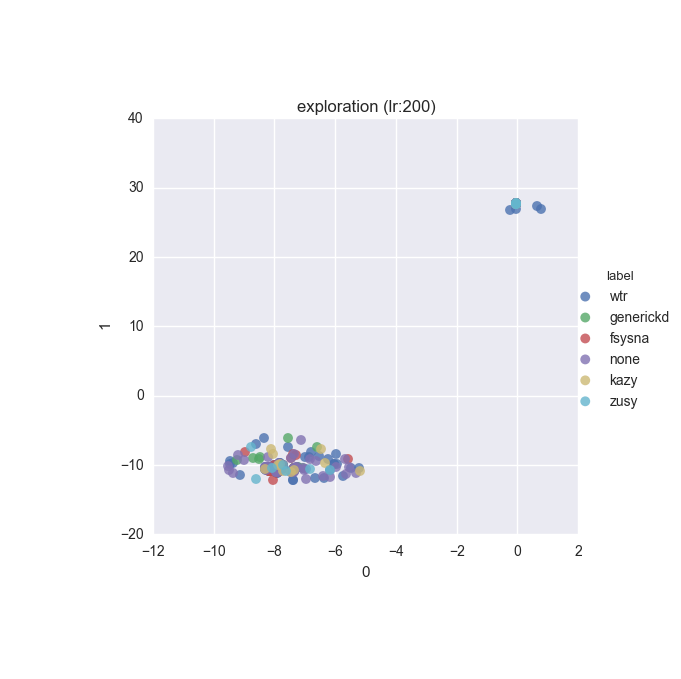
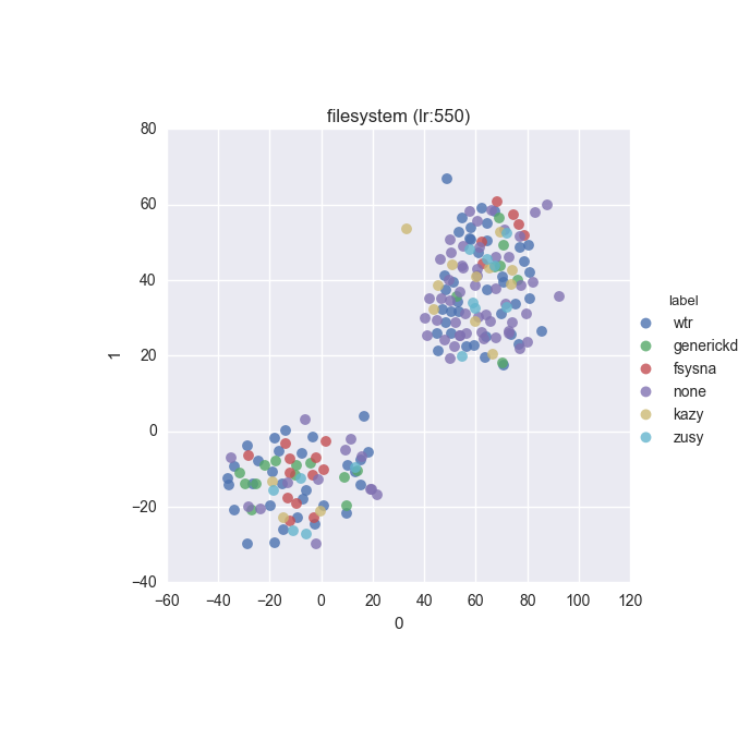
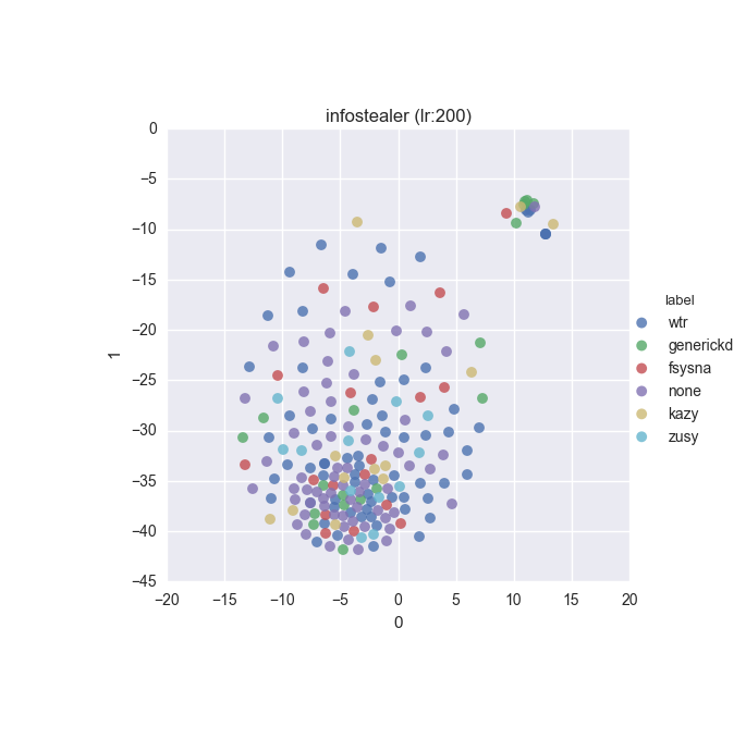
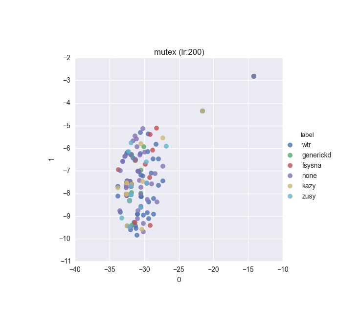
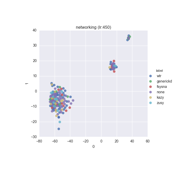
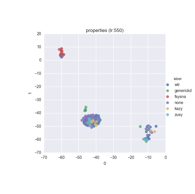
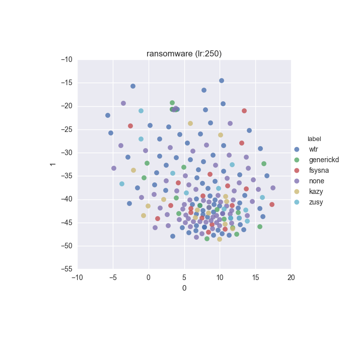
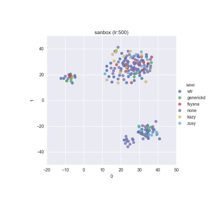
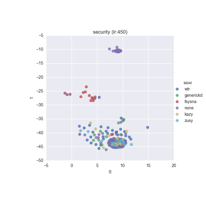
To inspect the data distribution with regard to selected features some visualisation technique has to be chosen. Due to high dimensionality of the feature space I decided to go with t-Distributed Stochastic Neighbour Embedding with variety of learning rates (200 to 600 in 50 increments were tested).

Additionally, due to overwhelming amount of labels (more colours than I can tell apart) I decided to put all labels with less than 10 instances into a single label called wtr. As a reminder, none label is assigned to samples which could not be identified as malware by VT analysis.

This snippet was used to produce presented below figures:

  from collections import Counter
  from modules.cuckooml.cuckooml import Loader
  from modules.cuckooml.cuckooml import ML

  loader = Loader()
  loader.load_binaries("../../sample_data/dict")

  ml = ML()
  ml.load_simple_features(loader.get_simple_features())
  ml.load_labels(loader.get_labels())

  # Remove uncommon labels
  new_labels = ml.labels.copy(True)
  a = Counter(list(ml.labels['label']))
  b = []
  for j in a:
      if a[j] < 10:
          b.append(j)
  new_labels = new_labels.replace(b, "wtr")

  # Pot groups for different learning rates
  for lr in [200, 250, 300, 350, 400, 450, 500, 550, 600]:
      for i in ml.SIMPLE_CATEGORIES:
          ml.visualise_data(data=ml.simple_feature_category(i),
                            labels=new_labels, fig_name=i,
                            learning_rate=lr)

  # Pot groups for different learning rates
  for lr in [200, 250, 300, 350, 400, 450, 500, 550, 600]:
      ml.visualise_data(data=ml.simple_features, labels=new_labels,
                        fig_name="all", learning_rate=lr)